Biostats
- PPV is highest with highest specificity
- mean, median, mode
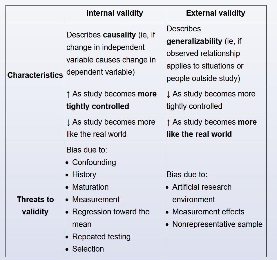
- internal vs external validity
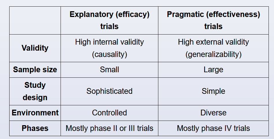
- explanatory vs pragmatic trials
- bias
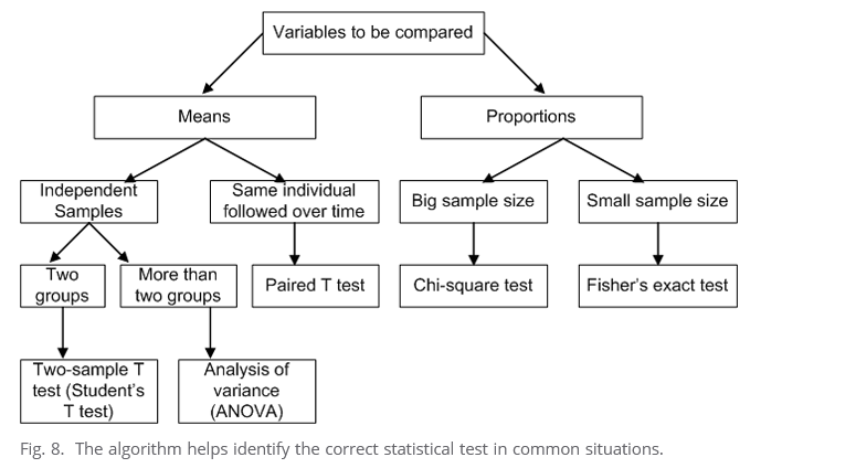
- comparison tests in statistics
- per year rates
- relative risk vs odds ratio
- coefficient of determination
- attributable risk
- receiver operating characterstics curve
- positive predictive value
- study designs
Likelihood ratio
The likelihood ratio (LR) is defined as the probability of a given test result occurring in a patient with a disorder compared to the probability of the same result occurring in a patient without the disorder.
The likelihood ratio (LR) is an expression of sensitivity and specificity that can be used to assess the value of a diagnostic test. The positive likelihood ratio (LR+) represents the value of a positive test result, and the negative likelihood ratio (LR-) represents the value of a negative test result.
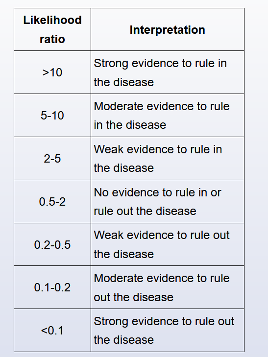
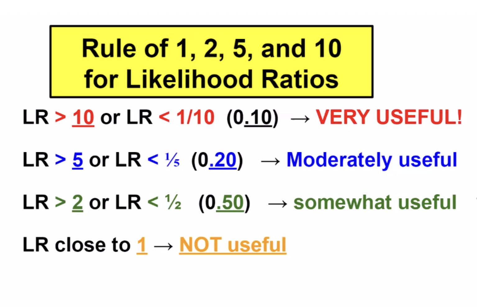
LRs can range from 0 to infinity. A test result with a LR >1 suggests disease presence; the higher the LR, the more likely the disease presence. A test result with a LR <1 argues against the disease; the lower the LR, the less likely the disease presence. There are general guidelines for LR interpretation (Table).
LRs are calculated from sensitivity and specificity:
- For a positive test result: Positive LR = sensitivity / (1 – specificity).
- For a negative test result: Negative LR = (1 – sensitivity) / specificity.
Just as sensitivity and specificity are independent of disease prevalence, LRs do not change with the prevalence of the disease. In addition, LRs can be used to calculate post-test odds (post-test odds = pre-test odds * LR), providing clinically relevant information for individual patients based on their pre-test odds of disease.
Other advantages of LRs are that they can be used with tests that have >2 possible test results and they can be used to combine the results of multiple diagnostic tests. For all these reasons, LRs would be the most appealing choice for the government agency officials in this scenario.
Predicative Values
Positive predictive value (PPV) refers to the probability that a positive test result correctly identifies an individual who actually has the disease. Negative predictive value (NPV) is the probability that a negative test result correctly identifies an individual without the disease. Although useful, both PPV and NPV depend on disease prevalence.
End of life
End-of-life care may involve discontinuation of ongoing therapies and/or shift to palliative therapies. This phase of treatment may begin when curative therapy is likely futile. Futility may be physiologic if the treatment is extremely unlikely to allow survival, or qualitative if it offers only minimal benefit at the cost of significant pain and suffering. When this point is reached, the primary goals of therapy shift toward minimizing discomfort, anxiety, and distress for the patient and family.
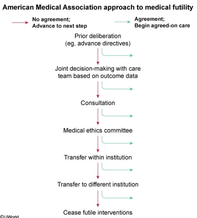
When the patient's family and medical team disagree about futility, a stepwise approach toward agreement should be implemented. First, family meetings, in which treatment and prognosis are discussed, are scheduled to promote joint decision-making. Second, for ongoing disagreement, a palliative care consultation or referral to the hospital ethics committee can help with arbitration. If resolution is still not reached, transferring the patient to another provider, either within the institution or to a different facility, can be considered.
Once the hospital ethics committee is involved and all providers have agreed that additional care is futile, then—and only then—should providers cease futile interventions in the absence of family agreement.
Risk reduction
The relative risk reduction (RRR) quantifies the proportion of risk reduction attributable to a specific intervention or exposure as compared to a control. RRR considers the risk for disease in the exposed/intervention group and the unexposed/control group as follows:
RRR = (risk in unexposed − risk in exposed) / (risk in unexposed)
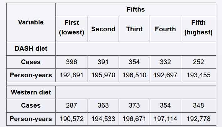
In this case, the exposed/intervention group is the DASH diet in the highest fifth, and the unexposed/control group is the DASH diet in the third fifth; the risks are reported in person-years (incidence densities). The risk of gout among subjects adopting a DASH diet in the third fifth (unexposed/control group) is 354 / 196,510 = 0.0018, or 1.8 per 1,000 person-years; the risk of gout among subjects adopting a DASH diet in the highest fifth (exposed group) is 252 / 193,455 = 0.0013, or 1.3 per 1,000 person-years. Therefore, the RRR is calculated as:
RRR = (1.8 per 1,000 person-years − 1.3 per 1,000 person-years) / 1.8 per 1,000 person-years
RRR = 0.5 / 1.8 = 0.28 (28%)
Alternately, RRR is frequently calculated by subtracting the relative risk (RR) from 1: RRR = 1 − RR. RR is the risk of developing a disease (eg, gout) in the exposed group (eg, DASH diet in highest fifth) divided by the risk of developing the same disease in the unexposed group (eg, DASH diet in third fifth). In this case, RR = 0.0013 / 0.0018 = 0.72 (72%) (Choice C). Therefore, RRR = 1 − 0.72 = 0.28.
This means that, compared to patients who adopt a diet DASH diet in the third fifth, patients who adopt a DASH diet in the highest fifth reduce their risk of gout by 28%.
Funnel Plot
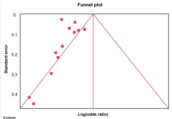
A funnel plot is helpful in assessing publication bias. Each study's treatment effect (on the x-axis) is plotted against a measure of that study's size or precision, usually using the standard error of the treatment effect (on the y-axis). The triangle is centered on a summary estimate of the treatment effect (eg, pooled estimate of odds ratio, usually in log scale) with its sides corresponding to standard errors. If there is no bias, any scatter between the study results should be due to sampling variation, and 95% of studies should lie within the triangle centered on the summary estimate and extending 1.96 standard errors on either side. Because a larger sample size is associated with increased precision, larger studies (more powerful) will be at the top and have a narrow spread whereas small studies will be scattered widely at the base of the triangle.
Funnel plots should be symmetric in the absence of study heterogeneity and publication bias. In this figure, however, there are no studies on the right side of the funnel. This asymmetry suggests publication bias (ie, studies showing null/increased effect of drug X on mortality are noticeably absent as they are less likely to have been published). Other possible explanations for asymmetry include heterogeneity, methodological anomalies, artifact, or chance.
A small sample size (low number of patients) in the drug X treatment arms would lead to more studies at the base of the triangle because such studies would have lower power and larger standard errors.
Intention to Treat
Intention-to-treat (ITT) analysis compares intervention groups in a randomized trial by including all subjects as initially allocated after randomization, regardless of what happens during the study period. The rationale is that if subjects are doing so poorly as to switch interventions or to drop out of the study, then their outcome should be attributed to that intervention. Therefore, ITT analysis is usually conducted to avoid the effects of crossover (eg, noncompliance to assigned intervention) and attrition (eg, loss to follow-up, drop-out), which may disrupt the benefit of randomization and introduce bias in the estimation of the effect of the intervention.
ITT analysis may lead to a more conservative estimate of the effect of the intervention. If attrition or crossover is significant, ITT analysis may be less likely to identify a statistically significant difference between interventions (shift toward the null hypothesis and reduced chances of false-positive conclusions). However, results will reflect the real effect of the intervention as intended in the population.
In this example, if subjects with more severe osteoarthritis drop out or cross over at a higher rate, even an ineffective intervention may appear beneficial if the analysis is conducted only on those who finished the protocol. Therefore, excluding subjects who were lost to follow-up or noncompliant to the assigned intervention introduces bias and may result in a statistically significant effect applicable only to subjects who completed the protocol. ITT analysis reduces bias by producing a more conservative but more valid estimate of the effect of using foot orthoses and motion control shoes as compared to motion control shoes alone.
In a per-protocol analysis, only data from subjects who completed the intervention originally allocated at randomization are analyzed. With as-treated analysis (a subtype of per-protocol analysis), subjects are evaluated based on the intervention they received rather than the intervention to which they were randomized. Therefore, the benefit of the randomization is lost. Usually, per-protocol analysis will overestimate the real effect of the intervention on the outcome.
Intention-to-treat is an important principle used in the analysis of randomized clinical trials. Intention-to-treat means that the patient's treatment status at the point of randomization is analyzed. If a patient who is assigned to the placebo group begins taking the medication assigned to the treatment group sometime after study initiation, or if a patient in the treatment group stops taking the prescribed medication, the data from these patients is still analyzed along with their original group. The value in the intention-to-treat approach is that it preserves the benefits of randomization and prevents bias due to selective non-compliance. Investigators may alternatively use the 'as treated' rule, which is the opposite of intention-to-treat (i.e. if a patient switches therapy they are counted as members of the new group during analysis).
Studies
A factorial study design (or fully crossed design) is a type of experimental study design that utilizes >2 interventions and all combinations of these interventions. In this study, there were 2 main interventions (antioxidant or glutamine supplementation) resulting in 4 possible study arms: glutamine supplementation, antioxidant supplementation, both, and neither (ie, placebo).
Although the authors randomized patients to these 4 arms, the results in the table provided are based on exposure or lack thereof to glutamine/antioxidant.
(Choice A) A crossover study is a type of experimental study design in which subjects are exposed to different treatments or exposures sequentially. The subjects cross over from one study arm to another and serve as their own controls.
(Choice B) A cross-sectional study is generally a type of observational study in which a specific population or group is studied at one specific point in time, therefore providing a cross section of the group at that particular time point. Unlike crossover or factorial studies, this is not experimental in nature.
(Choice D) A nested study (or nested case-control study) is a form of retrospective observational study in which subsets of controls are matched to cases and analyzed for the variables of interest.
(Choice E) A pragmatic study seeks to determine whether an intervention works in real-life conditions. This is contrasted with an explanatory study, which seeks to address whether an intervention works in optimal conditions and how/why it does or does not work. In general, randomized trials are considered explanatory, as randomization and other methods to control for confounders are not performed in the real world.
Noninferiority
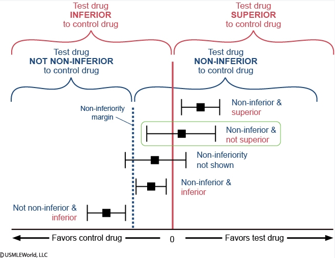
In the figure, each effect estimate for drug A is represented by a black square, with the horizontal black line representing the confidence interval.
The vertical red line centered at 0 splits the figure into 2 regions that compare drug A to warfarin: the region of superiority of drug A ("favors drug A") lies to the right and the region of inferiority of drug A ("favors warfarin") lies to the left. If the confidence interval crosses the red line, superiority cannot be proven. In superiority trials, the null hypothesis is that the effects of the drugs being compared are similar and the goal is to show that the new drug is different (better) than the comparator.
Similarly, the dotted blue line labeled "non-inferiority margin" also splits the figure into 2 regions that also compare drug A to warfarin: the region of non-inferiority of drug A lies to the right and the region of not non-inferiority of drug A lies to the left. In non-inferiority trials, the goal is to prove that a new drug is not unacceptably worse than a comparator (ie, the new drug should not be worse by more than an acceptable margin). The non-inferiority margin is used for this purpose and any effect estimate that lies entirely to its right is "non-inferior." The opposite of "non-inferior" is "not non-inferior"; any effect estimate that lies entirely to the left of the non-inferiority margin is "not non-inferior" (unfortunately, the terminology is confusing and relies on the use of double negatives). If the confidence interval crosses the margin, this implies that non-inferiority is not proven. Non-inferiority should be assessed prior to superiority.
Regarding drug A and myocardial infarction, the effect estimate lies entirely to the right of the non-inferiority margin, so drug A is non-inferior to warfarin. The confidence interval crosses the vertical red line at 0, so it cannot be said that drug A is superior to warfarin. In sum, drug A is non-inferior and not superior to warfarin in preventing myocardial infarction.
Analysis types
Sensitivity analysis refers to repeating primary analysis calculations after modifying certain criteria or variable ranges; the goal is to determine whether such modifications significantly affect the results initially obtained. With any study, a number of decisions are made based on certain assumptions or by consensus (eg, choosing 5-year rolling windows as opposed to 2- or 8-year rolling windows). If results of sensitivity analyses conducted with slight changes in certain variables (eg, changing rolling window period, changing cutoffs for average glucose levels by ±10%) are similar to the initial results, the investigators can be more confident of the robustness of their results.
In this case, patients with diabetes who had high fluctuations in glucose levels were excluded. If, on repeat analysis excluding those patients, the p-value for the association between average glucose levels and dementia remains statistically significant among the remaining patients with diabetes, this would further confirm the investigators' conclusions as it would make it less likely that high fluctuations in glucose levels explain the different hazard ratios obtained.
(Choice B) Linear regression models the linear relationship between a dependent variable and one or more independent variables. For example, multiple linear regression could be used to quantify the effects of alcohol use, tobacco smoking, and charred food consumption (independent variables) on the incidence of gastric cancer (dependent variable).
(Choices C and D) Propensity scoring typically weighs different variables (eg, severity of different comorbidities) in both the treatment and the control groups to ensure that these variables are balanced between both groups. An individual in the treatment group can be matched with an individual in the control group who has a similar propensity score. Matching can also be conducted based on similar variables (eg, age, sex) even in the absence of propensity scoring.
Time to event
Time-to-event data analysis is becoming more and more popular for analyzing follow-up studies and clinical trials. This type of analysis is called 'survival analysis'. A simple data layout for survival analysis is shown in Question #1. Rows are arranged by time intervals. In each row, data on the number of subjects who were present at the beginning of the time interval and the number who died during the interval are provided. Therefore probabilities of mortality/survival can be calculated for each time interval. For example, the probability for a patient to survive one additional month once he/she already survived the first two months of chemotherapy would be taken from the row for 2-3 months and calculated as 93% given that 7% of patients died during that interval (alternately, this result can be obtained by calculating the number of patients alive at the end of the interval, 170 - 12 = 158, and dividing that value by the number of patients alive at the beginning of the interval: 158/170 = 0.93 or 93%). Cumulative probability can be calculated by multiplying individual probabilities. For example, the probability that a patient on the new regimen would survive at least 3 months is the product of three probabilities obtained from the first three rows: 0.90_0.94_0.93 (given that 100% – 10% = 90% for 0-1 months, 100% – 5.6% = ~94% for 1-2 months, and 100% – 7% = 93% for 2-3 months).
It is important to understand that survival analysis accounts not only for the number of events in both groups, but also for the timing of the events. Despite the fact that two-year mortality risk is the same for both groups in Question #2, the patients in the treatment group may on average live longer than the patients in the placebo group. For example, the median survival time may be 3 months for the placebo group and 9 months for the treatment group. Therefore, in Question #2 time-to-event analysis could explain the conclusion that treatment was effective despite equal mortality at two years..
A survival plot represents a graphical description of survival analysis. An example is shown in Question #3. The concept of a latent period is demonstrated in this case. Latency is a very important issue to consider in chronic disease epidemiology. The latent period between exposure and the development of an outcome is relatively short in infectious diseases. In chronic diseases (e.g., cancer or coronary artery disease), however, there may be a very long latency period. In Question #3, at least three years of continuous exposure to multivitamins are required to reveal the protective effect of the exposure on cardiovascular outcomes. On the survival plot, you can clearly see that the survival curves run parallel to each other for three years (the latent period), and then begin to separate at the 3rd year of follow-up. Overall relative risk is not statistically significant, because it is 'diluted' by the years of latency, although the relative risk for the 5th year of follow-up, when isolated, clearly demonstrates the beneficial effect of therapy.
Organ donation
Organ donation is a difficult subject to bring up when dealing with grieving families. It requires excellent communication skills as well as extensive knowledge of the donation process to address any misconceptions or answer any questions the family might have. The role of the requestor is typically reserved for a trained Organ Procurement Organization (OPO) staff member, but can also be a treating physician who has undergone specialized training for this role. If not initiating the request for organ donation, physicians can play an important role in explaining the meaning of brain death and in being present and supporting the OPO staff when the option of organ donation is presented. This can be critical to the family's understanding and willingness to consider organ donation.
Physicians may have concerns that the family of the donor is too grief-stricken to consider donation or has religious beliefs that would preclude it. However, a treating physician cannot unilaterally decide whether a family should be approached regarding organ donation. Instead, the physician should work with the OPO staff to develop a plan to inform the family of the option for donation while respecting the family's beliefs.
Multiplicity
The hypothesis testing process requires that error rates (eg, type I and type II errors) be defined a priori. Type I error (alpha) is the probability of rejecting a null hypothesis when the null hypothesis is true. Conducting multiple independent hypothesis tests without proper adjustment to the alpha level increases the rate of type I error. This means that, when evaluating multiple secondary endpoints (eg, fasting plasma glucose, proportion of subjects reaching A1c <7.0%, changes in renal parameters), there is a higher probability of erroneously finding a statistically significant result with one of these endpoints (eg, higher likelihood of type I error) due to chance alone. This phenomenon is known as the multiplicity, or multiple testing, problem.
In general, the rate for type I error will increase depending on the alpha level for individual tests and the number of independent tests. For example, the rate for type I error in a study attempting to evaluate 5 secondary endpoints would be 23%, whereas the classically accepted value is usually set <5% (statistically significant p-value). The alpha level or p-value is sometimes adjusted to account for the multiple testing problem.